 Lavik
LavikMigrate Your 300-Node Redis Cluster to Just 3 Lavik Nodes
Why keep buying servers for RAM? Lavik combines NVMe SSD capacity with throughput above Redis on DRAM. Explore the architecture, benchmarks and economics of a 300-to-3 consolidation.
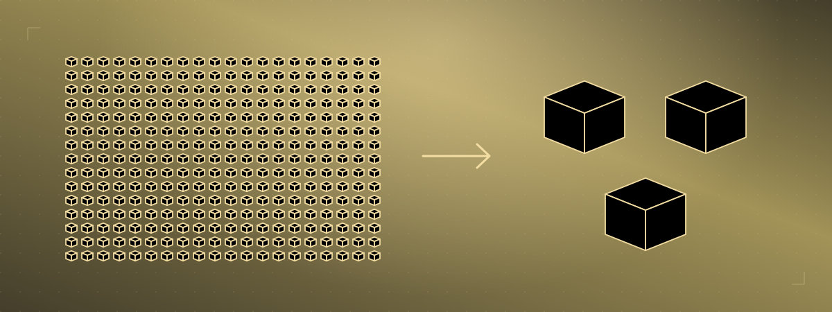
Memory is full. CPU still has room. Yet the next increase in retained data means another Redis shard, another replica, and another pair of servers to operate. For a capacity-bound application, that is an expensive way to grow. Lavik changes the resource that determines capacity: application values live on NVMe SSD, served by an engine that measured 1.14 million GETs per second—faster than Redis on DRAM in the published comparison. That combination opens a much more attractive design: consolidate a memory-bound fleet onto a few storage-dense hosts, with room for the next generation of agent state.[13][1]
1. Agents need more state—and fast access to it
A human-facing application might retain a profile, a session and a set of features per user. An agent application can retain all of these for a research assistant, a coding assistant and multiple background workers acting on that user’s behalf. Each agent accumulates execution state, observations and working context. An agent that runs occasionally may still need its state immediately when it resumes. Capacity grows with the number of agents, the size of their state and how long it remains useful; request volume does not have to grow at the same rate.[1]
At one billion agents, just 1 KB of features each produces approximately 1 TB of values. Increase that to 10 KB and the dataset reaches 10 TB; at 100 KB, it reaches 100 TB, before keys, indexes or replication. Applications still need low-latency reads and updates through familiar Redis clients and data structures. Keeping every retained value in expensive DRAM makes that combination harder to afford. Lavik is designed to make NVMe SSD capacity practical for those latency-sensitive workloads.[1][6]
| Bytes per agent | Unique value payload | Three copies, values only |
|---|---|---|
| 1 KB | 1 TB | 3 TB |
| 10 KB | 10 TB | 30 TB |
| 100 KB | 100 TB | 300 TB |
2. Stop adding servers just to add memory
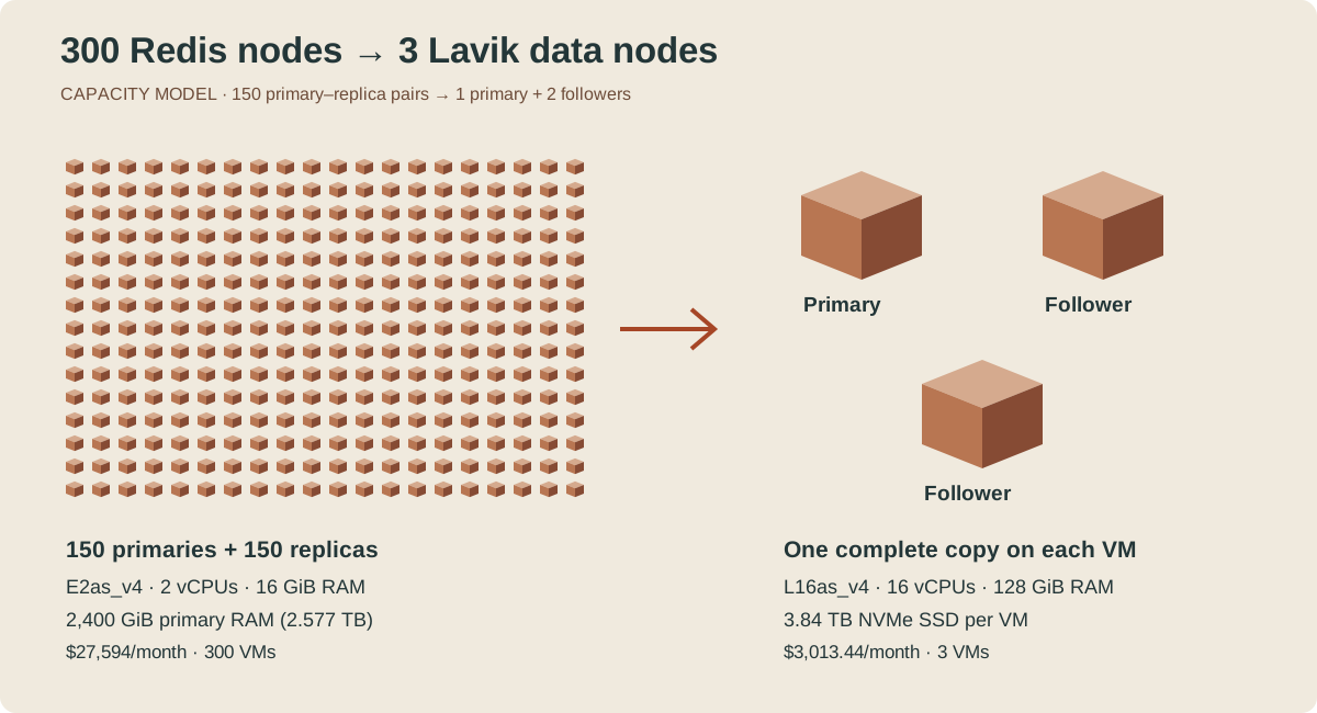
Consider 300 Standard_E2as_v4 Azure VMs, each with two vCPUs and 16 GiB RAM, arranged as 150 primaries and 150 replicas. The fleet buys 600 vCPUs and 4,800 GiB of RAM, with 2,400 GiB on the primary side. When memory fills first, expanding this fleet buys additional CPU, networking and operating systems largely to obtain more RAM. The application may need more retained profiles or longer session lifetimes without needing proportionally more compute. This is the central opportunity for Redis cost optimization: choose storage density independently of the processors needed to serve traffic.[1][28]
Use the same Azure region and purchasing model for both deployments: East US 2, Linux pay-as-you-go, in US dollars. Microsoft’s retail rate is $0.126 per hour for Standard_E2as_v4 and $1.376 per hour for Standard_L16as_v4. At 730 hours per month, 300 Redis VMs cost $27,594, while three Lavik VMs cost $3,013.44. The Lavik VM includes 16 vCPUs, 128 GiB RAM and 3.84 TB of local NVMe SSD. That puts the same cloud provider’s published VM prices behind the consolidation argument.[27][29][1]
Adding flash does not automatically solve the latency problem. Redis describes Flex’s flash access in milliseconds and advises against broad access patterns, large working sets and frequent movement between RAM and flash. For an application with a sub-millisecond latency budget, a millisecond flash path is too slow. Agent workloads that repeatedly revisit different profiles and contexts make this distinction consequential: the storage engine needs to serve a large dataset efficiently even when accesses spread beyond RAM.[25][26]
The monthly VM bill falls by $24,580.56—89.1%—and the annualized saving is $294,966.72. Lavik’s three VMs provide 48 vCPUs and 384 GiB RAM across the fleet, with NVMe SSD supplying the data capacity. Redis’s 300 VMs provide 600 vCPUs, much of which a memory-bound workload may not need. This is the economic benefit of storage density: pay for the compute needed to handle requests, then use SSD capacity to retain the data. The table prices self-hosted VMs for both systems; OS disks, backups and traffic are additional deployment costs.[1][27]
| Deployment | USD / VM-hour | Monthly USD | Annual USD | USD / million operations at 1M average QPS |
|---|---|---|---|---|
| Redis · 300 × Standard_E2as_v4 | $0.126 | $27,594.00 | $331,128.00 | $0.01050 |
| Lavik · 3 × Standard_L16as_v4 | $1.376 | $3,013.44 | $36,161.28 | $0.00115 |
3. Build capacity around NVMe SSD
Build the Lavik capacity design from three Standard_L16as_v4 VMs. Each has 16 vCPUs, 128 GiB RAM and four 960 GB local NVMe devices, totaling 3.84 TB per VM. Run one Data process and one Meta voter on each VM, with one primary and two full followers. Each VM holds a complete copy of the dataset. This gives the deployment a straightforward shape: three data placements, three control-plane voters and NVMe capacity in each serving node.[1][29][6][11][7]
With a full copy on each VM, the single-copy capacity basis is 3.84 TB. The cost table uses that denominator, yielding $784.75 per TB-month for the three-VM fleet. Redis’s 150 primaries provide 2,400 GiB, or about 2.577 decimal TB, yielding $10,707.88 per TB-month. These are capacity-normalized VM costs before database overhead and operational free-space reserves. Replication places the same logical dataset across the three Lavik VMs; after one VM fails, two data copies and a Meta majority remain available for recovery and promotion.[1][27][28][29][11][7]
| Deployment | Single-copy capacity denominator | USD / TB-month |
|---|---|---|
| Redis · 300 × E2as_v4 | 2,400 GiB RAM (≈ 2.577 TB) | $10,707.88 |
| Lavik · 3 × L16as_v4 | 3.84 TB NVMe SSD | $784.75 |
Lavik uses DRAM where it has the most value on the request path: the key index, metadata and active buffers. Values use NVMe SSD capacity. This separates growth in value bytes from growth in index memory, which is particularly useful as agent profiles and retained context become larger. Size RAM from the application’s key count and key lengths, together with buffers, hugepages and replication backlog. In the published large-dataset experiment, a billion-key layout fits a 125.8 GiB host while its values occupy about a terabyte.[9][13]
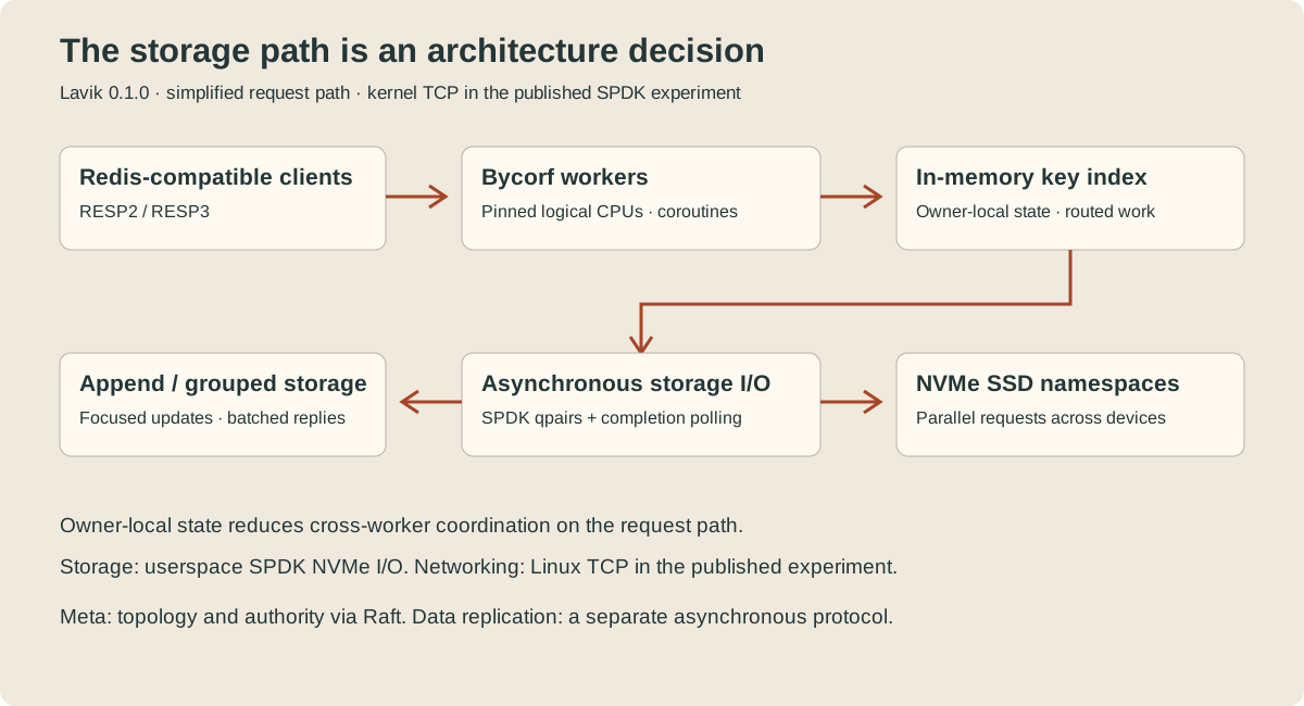
SPDK makes the storage path explicit. Lavik submits NVMe operations through userspace queue pairs and polls for completions, removing the kernel block-I/O submission path and its syscall and wakeup overhead. Asynchronous requests keep storage work in flight while workers make progress on other commands. Polling trades CPU time for prompt completion handling; queue depth, completion batching and CPU placement determine how effectively that time is used. Modern NVMe devices supply the parallel queues and internal concurrency. The engine must deliver enough independent work to exploit them.[4][5][13]
Lavik’s Bycorf workers use coroutines, owner-local mutable state and explicit dispatch between workers. While one command waits for storage, other runnable work can proceed. Ownership keeps common operations close to the state they modify and reduces coordination between cores. That matters at a million operations per second: small amounts of scheduling, synchronization or allocation overhead accumulate into substantial CPU demand. Designing execution and storage together lets Lavik use SSD parallelism without turning every I/O into a stalled request-processing thread.[6][8][9]
The optimizations extend through the request path. Eligible disk GETs can use an admitted index snapshot on the connection worker, avoiding owner dispatch when the fast path applies. Parsing handles batches of up to 128 commands, and small pipeline replies can coalesce into 64 KiB writes. Per-worker append streams avoid a staging-buffer allocation for every logical slot. Together, these choices reduce coordination, system calls and buffer overhead. The Redis-compatible interface stays familiar to applications; the implementation underneath is built around efficient concurrent storage access.[8][9]
Large objects receive the same attention. Lavik 0.1.0 supports grouped storage for Strings, Hashes, Sets, Lists, Sorted Sets and Streams. Large strings use 8 KiB segments, while collections use independently addressed groups. A focused operation can work on the relevant part instead of rewriting an entire large object. For an agent profile with frequently changing features and much larger retained state, that layout makes the difference between a small update and unnecessary work across the whole record. NVMe performance depends on both how I/O is scheduled and how much data each operation touches.[10]
4. Faster than Redis on DRAM—with values on SSD
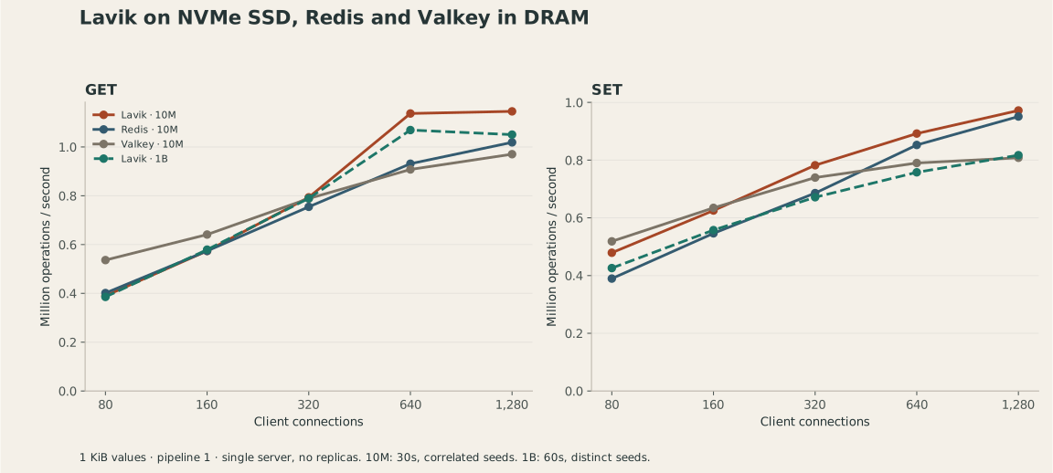
The direct benchmark compares Lavik 0.1.0 SPDK with Redis 8.10.2 and Valkey 9.1.2 on the same 16-vCPU Azure server. A separate load generator issues uniform random GETs and SETs over private networking, with 1 KiB values and pipeline depth one. Redis and Valkey serve their values from DRAM; Lavik uses its NVMe storage path. The table shows throughput and client-observed latency together, so readers can choose an operating point against their application’s latency budget.[13]
At 1,280 connections, Lavik delivers 1,145,772 GET QPS and 971,950 SET QPS. GET throughput is 12.5% higher than Redis and 18.1% higher than Valkey; SET throughput is 2.2% higher than Redis. Lavik’s GET P99 at that point is 3.999 ms, compared with Redis’s 4.415 ms. This is the architectural result that makes consolidation worth considering: NVMe-backed capacity can come with higher throughput than an in-memory server, rather than forcing the application to exchange performance for lower storage cost.[16][13]
| System / operation | QPS | Average | P50 | P95 | P99 | P99.9 |
|---|---|---|---|---|---|---|
| Lavik 0.1.0 SPDK GET | 1,145,772 | 1.117 | 1.031 | 1.511 | 3.999 | 7.135 |
| Lavik 0.1.0 SPDK SET | 971,950 | 1.317 | 1.119 | 2.783 | 4.479 | 7.199 |
| Redis 8.10.2 GET | 1,018,735 | 1.256 | 1.087 | 2.479 | 4.415 | 7.103 |
| Redis 8.10.2 SET | 951,053 | 1.346 | 1.135 | 2.943 | 4.511 | 7.231 |
| Valkey 9.1.2 GET | 970,288 | 1.319 | 1.119 | 2.511 | 4.415 | 7.455 |
| Valkey 9.1.2 SET | 808,103 | 1.583 | 1.455 | 2.559 | 4.047 | 7.199 |
Latency also depends on how hard a server is driven. At the billion-key operating point with 80 connections, Lavik delivers 385,514 GET QPS at 0.439 ms P99.9. At 640 connections, it reaches more than a million GETs per second. An infrastructure team can use these curves to select the throughput and tail-latency combination it needs. Keeping headroom for bursts is more useful than sizing a production deployment solely from the highest point on a throughput chart.[13]
The billion-key dataset contains 1.024 TB of raw values—about 7.6 times the server’s RAM—and reaches 1,069,126 GET QPS. Lavik’s performance therefore extends well beyond a memory-sized dataset. The smaller-instance results tell the same capacity story: on two vCPUs and 16 GiB nominal RAM, increasing the dataset from one million to 100 million 1 KiB values changes peak GET throughput from 215,521 to 215,463 QPS. SET retains 95.2% of its smaller-dataset peak. That is valuable for both a compact service and a large agent platform: capacity can grow without demanding a matching increase in serving nodes.[13][14]
Agent state also needs updates. In the separate io_uring YCSB experiment, Lavik processes 529,501 operations per second for a 50/50 read/update mix and 577,373 for a 95/5 mix. These are structured-record operations: HGETALL reads and LAVIK.HREPLACE updates against 100 million records with ten 128-byte fields. They show the relevance of Lavik’s design beyond a pure GET workload, including feature records whose contents change as an agent progresses through a task.[15]
| Lavik workload | Total QPS | READ P99.9 ms | UPDATE P99.9 ms |
|---|---|---|---|
| 50% HGETALL / 50% HREPLACE | 529,501 | 5.083 | 2.831 |
| 95% HGETALL / 5% HREPLACE | 577,373 | 1.818 | 1.578 |
One million operations per second corresponds to 86.4 billion operations per day if sustained. That level of measured serving performance, combined with NVMe storage density, makes a strong case for reevaluating a memory-bound fleet. Start with the actual traffic envelope—command mix, peak demand, bursts and latency target—and allocate compute to that envelope. Let NVMe SSD provide the capacity for everything the application needs to remember.[1][13]
5. Fewer nodes mean less cluster machinery
Memory-driven growth also expands the topology engineers must operate. Redis Cluster distributes 16,384 hash slots and uses a full-mesh cluster bus. Its specification gives each node N−1 outgoing and N−1 incoming bus connections. Across the cluster, that is N(N−1) initiated connections: 89,700 at 300 nodes, 359,400 at 600 and 999,000 at 1,000. These are cluster-bus connections, separate from application traffic. As agent state expands, adding memory through more nodes also increases the size of this coordination fabric.[2]
The cluster uses gossip, heartbeat probes and failure reports to maintain membership and health. Local failure suspicion must be reconciled with reports from other nodes; failover requires authorization and configuration epochs. During a network partition or rolling restart, engineers must understand which primaries, replicas and paths remain reachable. More members create more placements and relationships to diagnose, even when request-processing capacity is sufficient. The operating cost of a fleet includes this work as well as the VM bill.[2]
Resharding adds data movement, ownership changes and client redirects. Maintenance adds patching, restarts, monitoring and replica placement. A storage-dense Lavik deployment reduces the number of Data processes needed for capacity and gives each one room to grow. Lavik’s Meta service manages topology and authority, while native replication maintains followers. For a capacity-bound application, reducing the fleet addresses two expenses at once: the servers purchased for memory and the operational work that comes with managing them.[3][6][11][7]
6. Move the workload, keep the service requirements
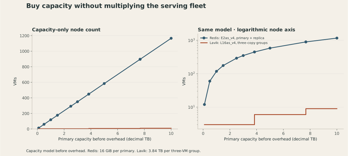
The strongest consolidation candidate is easy to recognize: memory pressure keeps forcing expansion while CPU utilization and traffic remain below the fleet’s serving capacity. Select a representative workload and size Lavik for its commands, key count, value distribution and busiest periods. A demanding tail-latency target or CPU-intensive command mix may need additional serving capacity. The architectural advantage remains the same: retained data no longer has to determine node count through DRAM capacity alone.[1][6]
Build availability into the deployment from the beginning. Place VMs in appropriate failure domains and keep Meta state on durable disks. Azure’s local NVMe is temporary storage, so pair replication across VMs with external backups. Measure serving latency with replication, expiration and reclamation active, then rehearse primary failure and follower rebuild at the intended dataset size. Lavik’s Meta uses Raft for topology and authority, while Data replication is asynchronous. Set the application’s recovery-point and recovery-time targets accordingly, then verify them through failover drills.[29][11][7][1]
Use RedisShake to move from the existing Redis deployment. Inventory commands and key shapes, create the managed Lavik target, copy the baseline and follow incremental changes. Reconcile key counts, values and expirations before cutover. Pause source writes for the final catch-up, switch clients, and keep a rollback procedure that accounts for new writes. The source shard count does not have to dictate the target’s physical layout. The linked migration guide provides release-pinned configuration and steps for turning the consolidation design into an executable migration.[12]
7. Give agent state room to grow
When retained state grows from 1 TB to 10 TB and beyond, the cost of each additional terabyte becomes a product constraint. Lavik offers a different foundation: a Redis-compatible NVMe key-value store with measured throughput above Redis on DRAM, efficient large-object storage and an Apache 2.0 open-source license. Start with the commands your application uses, load a representative dataset and measure the latency budget that matters to your users. From 300 Redis nodes to three Lavik nodes, the opportunity is to build around the workload’s real compute demand—and give its data room to grow.[6][10][13][1]
Benchmark and sizing notes
Benchmark setup: Azure Standard_L16aos_v4, Japan West zone 2, AMD EPYC 9V74, 16 logical CPUs (eight physical cores with SMT), 125.8 GiB RAM and six 1.92 TB NVMe devices. The F32als_v6 client uses 16 threads over private accelerated mlx5 networking and Linux TCP. Ten-million-key windows run for 30 seconds with correlated seeds; billion-key windows run for 60 seconds with distinct seeds. Lavik uses 8 GiB of hugepages, defrag enabled and 16 completions per poll. Selected Redis I/O-thread counts are 16 for GET and SET; Valkey uses 16 for GET and eight for SET. All runs use a single server without Data replicas; Redis and Valkey disable AOF and scheduled snapshots.[13]
Measurement details: each curve point is one measured window. Latencies come from whole-window memtier results; P95 is decoded from the embedded HDR histogram. The mixed-workload experiment uses io_uring, 12 Lavik workers plus four system/IRQ CPUs, 256 client workers and 300-second windows without replicas. These reports cover the workloads shown; production selection should also measure the application’s own value sizes, command mix and replicated tail latency.[16][13][15]
Sizing and cost basis: the Azure comparison uses 300 E2as_v4 VMs versus three L16as_v4 VMs, with Linux pay-as-you-go prices in East US 2 and 730 hours per month. Annual cost is 12 monthly periods. Capacity normalization counts one logical copy: 2,400 GiB of Redis primary RAM and 3.84 TB of Lavik NVMe SSD, both before overhead. The throughput results use the separate L16aos_v4 benchmark configuration described above. Cost per million operations assumes an average 1 million QPS. VM prices exclude managed disks, external backups, traffic, staffing and taxes.[1][27][28][29][13]